ElasticSearch的Agg聚合检索
前言
ES的一个很重要的功能是它的聚合分析能力,通过对搜索条件匹配到的文档进行聚合,可以获取到如最小值、最大值、某类数据的文档数等等。
文章介绍了如何使用一些常见的聚合,及一些需要关注的点。
创建测试索引
1、创建索引 my_products
PUT http://127.0.0.1:9200/my_products
使用动态配置
2、索引文档:
POST http://127.0.0.1:9200/my_products/_bulk

{ "index": { "_id": 1 }}
{ "productID" : "XHDK-A-1293-#fJ3","desc":"My little iPhone", "createTime":"2023-08-16", "price": 10, "status":true}
{ "index": { "_id": 2 }}
{ "productID" : "KDKE-B-9947-#kL5","desc":"My big iPad", "createTime":"2023-08-18", "price": 20, "status":true}
{ "index": { "_id": 3 }}
{ "productID" : "JODL-X-1937-#pV7","desc":"My medium MBP", "createTime":"2023-08-20", "price": 30.5, "status":false}
json内容后面加个空行,不然报错。
3、通过下面search可以确认文档已经被索引成功。
GET http://127.0.0.1:9200/my_products/_search

{
    "query":{
        "match_all":{}
    }
}
Agg类型
ES的agg聚合可以被分成3种类型:
1、Metric agg:指标度量分析,例如总数、平均值等。
2、Bucket agg:基于字段的值、范围等将文档分组到不同的bucket中。
3、Pipeline agg:基于其它的聚合进行的数据再次聚合计算。
Metric agg
Metric 是进行指标的度量,如最小值、最大值、前3、前10等。
它可以基于搜索的文档、也可以基于聚合的bucket进行分析。
数值类型(输出数字)的聚合比较常见,它包括了单值输出类型和多值输出类型。
举例1:
对于获取商品信息的最低价格聚合:
GET http://127.0.0.1:9200/my_products/_search

{
    "size":0,
    "aggs": {
      "minPrice":{
        "min": {
          "field": "price"
        }
      }
    }
}
minPrice为agg的名称,min为关键词。size为0表示不返回hits,只返回聚合结果。
结果如下(忽略部分输出),最低价为10:
{
	"hits": {
		"total": {
			"value": 3,
			"relation": "eq"
		},
		"max_score": null,
		"hits": []
	},
	"aggregations": {
		"minPrice": {
			"value": 10
		}
	}
}
如果将 min 换成 stats 关键词,便是一个多值聚合,它将返回包括 min、max、sum、count 和 avg。
举例2:
每种商品状态下的前2个最高价格:
可以先按状态分桶(分桶后面会介绍),然后使用Top hit agg,进行价格排序,获取前2个。
GET http://127.0.0.1:9200/my_products/_search

{
  "size":0,
  "aggs": {
    "top_aggs":{
      "terms": {
        "field": "status"
      },
      "aggs": {
        "top_price":{
          "top_hits":{
             "sort": [
              {
                "price": {
                  "order": "desc"
                }
              }
            ],
			"_source":["status", "price"],
            "size": 2
          }
        }
      }
    }
  }
}
top_aggs和top_prices分别定义了agg的名称 ;terms和第二个aggs同层; _source 指定返回的字段;size指定每个bucket内的top数量;
结果如下:
{
  "aggregations": {
    "top_aggs": {
      "doc_count_error_upper_bound": 0,
      "sum_other_doc_count": 0,
      "buckets": [
        {
          "key": 1,
          "key_as_string": "true",
          "doc_count": 2,
          "top_price": {
            "hits": {
              "total": {
                "value": 2,
                "relation": "eq"
              },
              "max_score": null,
              "hits": [
                {
                  "_index": "my_products",
                  "_id": "2",
                  "_score": null,
                  "_source": {
                    "price": 20,
                    "status": true
                  },
                  "sort": [
                    20
                  ]
                },
                {
                  "_index": "my_products",
                  "_id": "1",
                  "_score": null,
                  "_source": {
                    "price": 10,
                    "status": true
                  },
                  "sort": [
                    10
                  ]
                }
              ]
            }
          }
        },
        {
          "key": 0,
          "key_as_string": "false",
          "doc_count": 1,
          "top_price": {
            "hits": {
              "total": {
                "value": 1,
                "relation": "eq"
              },
              "max_score": null,
              "hits": [
                {
                  "_index": "my_products",
                  "_id": "3",
                  "_score": null,
                  "_source": {
                    "price": 30.5,
                    "status": false
                  },
                  "sort": [
                    30
                  ]
                }
              ]
            }
          }
        }
      ]
    }
  }
}
结果分为两个bucket,一个是status为true的,一个好是status为false的,分别返回它们中price靠前的2个文档。
Bucket agg
基于字段的值、范围等将文档分组到bucket中。
在上面的Top hit例子中,已经提到了关于bucket聚合,可以理解成,它是按类型或者时间区间或者值区间等等分组,将相同类型的一组文档放到1一个桶内。
比较常见的一种分桶方式是terms agg,它是通过文档的某个字段,将值相同的放到1个桶内,默认会返回10个桶的大小,桶的排序使用doc_count数进行倒序。
举例:
参考上面的例子,将不同类型的商品进行分组
GET http://127.0.0.1:9200/my_products/_search

{
  "size":0,
  "aggs": {
    "status_aggs":{
      "terms": {
        "field": "status"
      }
    }
  }
}
status_aggs为bucket的名称,terms为关键词
结果如下:
{
  "aggregations": {
    "status_aggs": {
      "doc_count_error_upper_bound": 0,
      "sum_other_doc_count": 0,
      "buckets": [
        {
          "key": 1,
          "key_as_string": "true",
          "doc_count": 2
        },
        {
          "key": 0,
          "key_as_string": "false",
          "doc_count": 1
        }
      ]
    }
  }
}
省略了部分输出,每个bucket里包括了分桶的唯一值key和数量doc_count。
Pipeline agg
基于其它的聚合进行的数据再次聚合计算。
例如:
在按status分组后,取每个桶的最高价,最后将每个桶的最大值再取一个最终的最高价:
示例仅为了演示功能
http://127.0.0.1:9200/my_products/_search

{
  "size":0,
  "aggs": {
    "termsAgg":{
      "terms": {
        "field": "status"
      },
      "aggs": {
        "minPrice":{
          "min":{
             "field": "price"
          }
        }
      }
    },
    "maxPriceOfAll": {
      "max_bucket":{
        "buckets_path": "termsAgg > minPrice"
      }
    }
  }
}
首先terms分桶命名termsAgg;
每个桶内使用matrics agg取最大的价格,命名为minPrice;
最后在所有桶中取一个最大值,命名maxPriceOfAll,与size同层,max_bucket为关键词,buckets_path指定了聚合数据路径。
结果如下(省略部分结果):
{
  "aggregations": {
    "termsAgg": {
      "doc_count_error_upper_bound": 0,
      "sum_other_doc_count": 0,
      "buckets": [
        {
          "key": 1,
          "key_as_string": "true",
          "doc_count": 2,
          "minPrice": {
            "value": 10
          }
        },
        {
          "key": 0,
          "key_as_string": "false",
          "doc_count": 1,
          "minPrice": {
            "value": 30
          }
        }
      ]
    },
    "maxPriceOfAll": {
      "value": 30,
      "keys": [
        "false"
      ]
    }
  }
}
Terms agg注意点
Terms分桶聚合是比较常见的,它有一些出入参数需要我们注意,用不好,可能就会获取到不精确的结果,当然这也是结果和性能的一种平衡和取舍,也即trade-off。
size 入参
默认情况下,terms agg共返回10个bucket大小,可以通过size参数指定返回的大小,不过它受限于 search.max_buckets 配置(默认65535),所以size不要设置超过这个数,一般也不需要。
更大的size意味着需要更多的内存和计算。
shard_size 入参
分桶聚合时,会根据每个分片返回的聚合结果,在coordinating node(协调节点)进行汇总,该参数用于配置每个分片返回的terms(桶)数量,可以提高精确度。默认 shard_size = size * 1.5 + 10。
该参数主要用于解决1个桶在某一个分片上有很多文档,但是在所有分片上会低于size的大小,这个桶不应该被返回,但有可能被返回了。
shard_size的大小不能设置小于size,因为这并不合理,如果这样配置的话,ES会将shard_size修改成等于size。
terms agg不精确原因
了解了这两个参数,那为什么Terms agg在大数据量的情况下是不精确的呢?
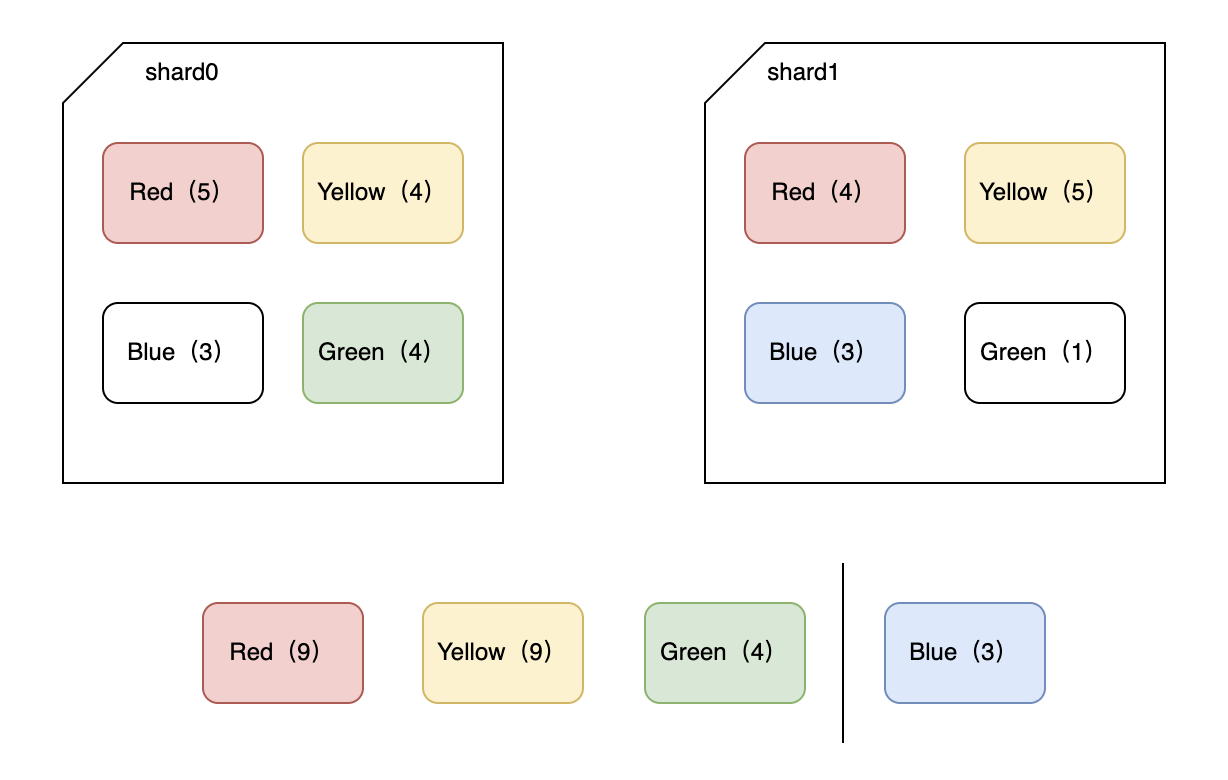
如图所示,有两个主分片shard0和shard1,索引文档有个颜色字段,每个分片上有一些不同颜色的文档,如图括号内数值所示。
在shard_size被设置成3的时候,当我们按颜色terms agg聚合,那么每个分片会返回数量top3的结果:
1,shard0提取颜色数靠前的3个,分别是red、yellow、green,对应文档数分别是5、4、4。
2,shard1提取颜色数靠前的3个,分别是red、yellow、blue,对应文档数分别是4、5、3。
那么在协调节点进行计算的时候,便会返回red、yellow和green,分别文档数为:9、9、4。
但是,实际结果应该是Blue(6)排第3位。
所以结果错了,原因主要是协调节点只获取到了每个分片的部分数据,无法获取全貌数据导致。
解决办法(提高精确度):
1、在数据量不大的情况下,可以将数据放到1个主分片上。
2、增加shard_size,将每个分片返回的bucket调大,但要注意会增加计算成本。
doc_count_error_upper_bound 出参
该结果表示:被遗漏的term分桶中,可能包含的文档最大值,是一个粗估值。
sum_other_doc_count 出参
该结果表示:当结果有很多桶时,ES默认返回文档数量大的前10个桶,这个参数值表示应该返回的所有桶的文档总数减去实际返回的桶内的所有文档总数,有可能是协调节点不能填充到size大小或者分片不能填充到shard_size大小。
出参示例
通过示例加强这两个参数的理解,测试如下:
1、创建索引 test_terms:
PUT http://127.0.0.1:9200/test_terms

{
  "settings": {
    "number_of_shards": 2,
    "number_of_replicas": 0
  },
  "mappings": {
    "properties": {
      "tags" : {
        "type": "keyword"
      },
      "value" : {
        "type": "integer"
      }
    }
  }
}
指定tags为keywrod类型,可被聚合。
2、索引文档数据
数据量如下:
routing:A
tags:a - count:6
tags:b - count:4
tags:c - count:4
tags:d - count:3
routing:B
tags:a - count:6
tags:b - count:2
tags:c - count:1
tags:d - count:3
POST http://127.0.0.1:9200/test_terms/_bulk

{"index":{"routing":"A"}}
{"tags":"a","value":1}
{"index":{"routing":"A"}}
{"tags":"a","value":2}
{"index":{"routing":"A"}}
{"tags":"a","value":3}
{"index":{"routing":"A"}}
{"tags":"a","value":4}
{"index":{"routing":"A"}}
{"tags":"a","value":5}
{"index":{"routing":"A"}}
{"tags":"a","value":6}
{"index":{"routing":"A"}}
{"tags":"b","value":1}
{"index":{"routing":"A"}}
{"tags":"b","value":2}
{"index":{"routing":"A"}}
{"tags":"b","value":3}
{"index":{"routing":"A"}}
{"tags":"b","value":4}
{"index":{"routing":"A"}}
{"tags":"c","value":1}
{"index":{"routing":"A"}}
{"tags":"c","value":2}
{"index":{"routing":"A"}}
{"tags":"c","value":3}
{"index":{"routing":"A"}}
{"tags":"c","value":4}
{"index":{"routing":"A"}}
{"tags":"d","value":1}
{"index":{"routing":"A"}}
{"tags":"d","value":2}
{"index":{"routing":"A"}}
{"tags":"d","value":3}
{"index":{"routing":"B"}}
{"tags":"a","value":1}
{"index":{"routing":"B"}}
{"tags":"a","value":2}
{"index":{"routing":"B"}}
{"tags":"a","value":3}
{"index":{"routing":"B"}}
{"tags":"a","value":4}
{"index":{"routing":"B"}}
{"tags":"a","value":5}
{"index":{"routing":"B"}}
{"tags":"a","value":6}
{"index":{"routing":"B"}}
{"tags":"b","value":1}
{"index":{"routing":"B"}}
{"tags":"b","value":2}
{"index":{"routing":"B"}}
{"tags":"c","value":1}
{"index":{"routing":"B"}}
{"tags":"d","value":1}
{"index":{"routing":"B"}}
{"tags":"d","value":2}
{"index":{"routing":"B"}}
{"tags":"d","value":3}
指定路由,让其可以分配到2个主分片上。可以通过GET /_search?routing=A/B 分别查看A/B上的文档数据。
3、聚合检索,size和shard_size都设置成3:
http://127.0.0.1:9200/test_terms/_search

{
  "size": 0,
  "aggs" : {
    "tags_count" : {
      "terms": {
        "field": "tags",
        "size": 3,
        "shard_size": 3
      }
    }
  }
}
结果如下:
{
  "took": 202,
  "timed_out": false,
  "_shards": {
    "total": 2,
    "successful": 2,
    "skipped": 0,
    "failed": 0
  },
  "hits": {
    "total": {
      "value": 29,
      "relation": "eq"
    },
    "max_score": null,
    "hits": []
  },
  "aggregations": {
    "tags_count": {
      "doc_count_error_upper_bound": 6,
      "sum_other_doc_count": 7,
      "buckets": [
        {
          "key": "a",
          "doc_count": 12
        },
        {
          "key": "b",
          "doc_count": 6
        },
        {
          "key": "c",
          "doc_count": 4
        }
      ]
    }
  }
}
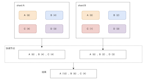
处理流程,如图所示:
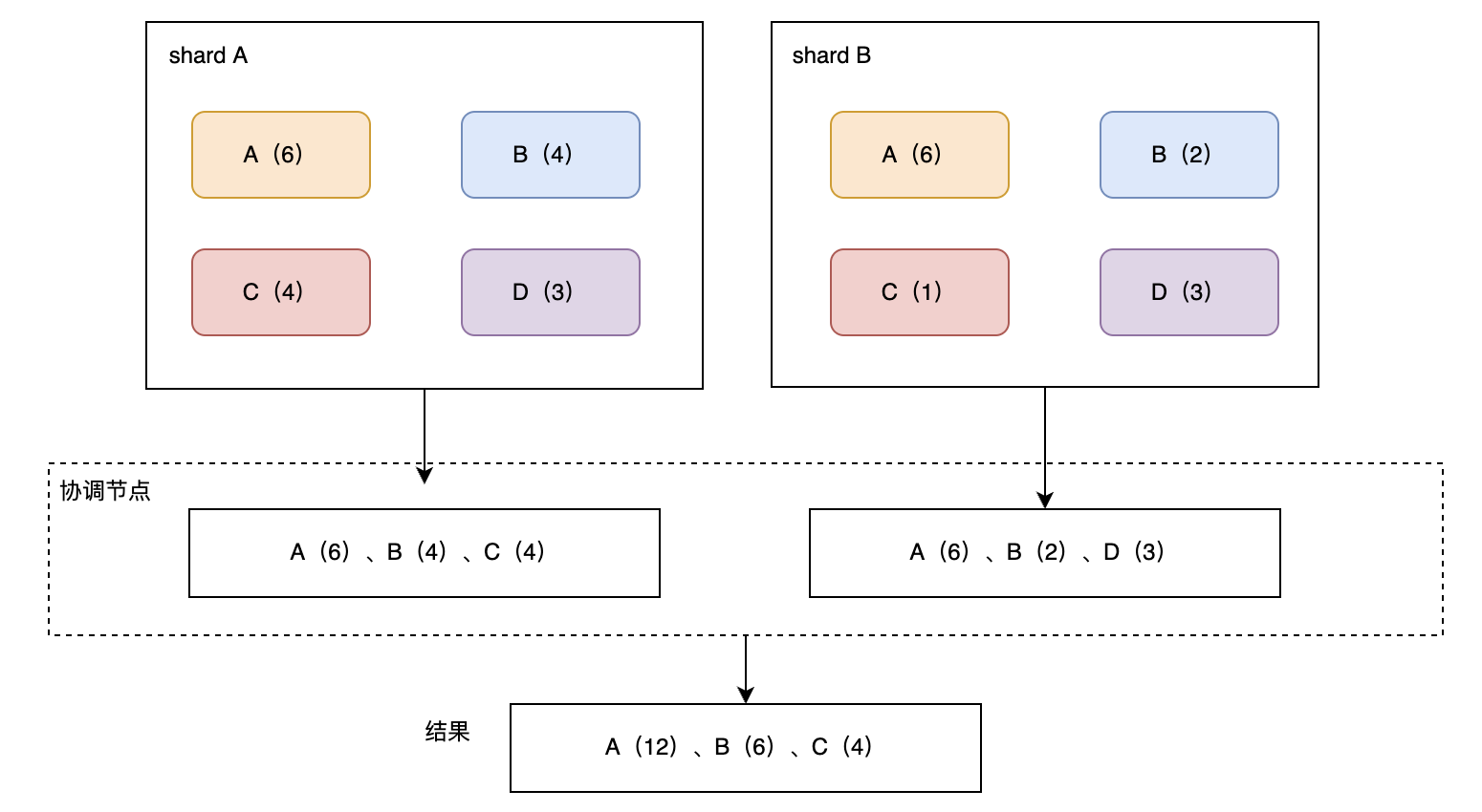
其中:
“doc_count_error_upper_bound”: 6(分片A取回的最小的为4 + 分片B取回的最小的为2);
“sum_other_doc_count”: 7(总共29个文档 - 返回的22个文档 = 7);
如果不指定shard_size,那么示例中doc_count_error_upper_bound为0,因为shard_size按默认值: size*1.5 +10计算。sum_other_doc_count为5,因为size等于3,有1个桶key=C未返回。
总结
ES的聚合分析是相对高效的,通过倒排索引加上Doc values进行聚合。
总共分为3类聚合,包括Metrics、Bucket、Pipeline,它们分别适用于不同的聚合场景。
其中Bucket聚合中有一个terms聚合,在大数据量多分片的情况下可能不够精确,可以通过将主分片设置成1或者增大shard_size来提高精确度。也通过示例演示了terms aggs下doc count error的情况,以便加深理解。